NFL Sports Analysis

Applying Post Prediction Inference to the NFL: How We Strive to Reinvent Sports Analysis

By: Jonathan Langley, Sujeet Yeramareddy, and Yong Liu

1.Introduction

For our 180B project, we decided to use our domain methodology of postpi (post prediction inference) and apply it to sports analysis based on NFL games. We are designing a model that can predict the outcome of a football game, such as which team will win and what the margin of their victory will be, and then correcting the statistical inference for selected key features. The main goals of our investigation is discerning which features most strongly determine the victor of a football game, and subsequently which features provide the most significant means of inferring the margin of that victory. For example, does the home field advantage give a 50% higher chance of winning by 7 points? Is the comparative offense to defense rating the most critical factor in securing a win? Does or does not weather play a statistically significant part in influencing margin of victory? These are just some of the questions we have brought up and seek to answer during the course of our research, and by conducting this project we are attempting to revolutionize the way NFL analytics are conducted via a more accurate statistical method of inference, postpi.

2.Data Collection

Data source: https://stathead.com/football/

For the data collection portion we used this website to manually copy and paste NFL game data from the 2000 season to 2021 season for each individual feature. This process was quite tedious because we were only able to access 100 rows of the data at a time. Additionally, we had to obtain the data for many game features for all NFL games therefore it took longer than expected and required us to split up the simple, yet time-consuming, task. The features that we included in our dataset included, but are not limited to, first downs, passing, rushing, defense, penalties, and temperature.

3.Data Cleaning

We used game characteristics such as teams playing, date of game, week of season, and more to merge the many individual datasets together so that we have one big dataset that included over 60 columns representing 5600+ NFL games in the past 21 years. It is important to note that our dataset actually includes over 10,000 rows because each game must be represented by 2 entries to avoid model bias in Spread prediction. The dataset contains two columns that denotes which NFL team is categorized as “Tm” and “Opp” which represent the order of each team’s statistics for the team. By swapping the team in these columns we can represent the same game twice which allows us to include positive and negative spreads in our dataset for our model to learn on.

Once obtaining this large dataset, our next task was to clean our dataset so that our data is easier to explore, analyze, and use to predict.

1. The first step we took was to fix specific columns in our dataset such as "Home" and "Result". The "Home" column originally had an @ symbol when it was a Home game for the team in the "Opp" column, and missing otherwise, therefore we chose to replace the @ values with a 0 to transform this to a binary column that represents when the team in the "Tm" columns was home.
2. The second step we took was to fix the "Result" column was originally in the format of a string like "W 12 - 9" which represents the score of the NFL game in the format "TmOutcome TmScore - OppScore” based on the teams in each of these columns. We took this column and used string manipulation to convert it into a column named Spread which is our response variable that we are trying to predict. Spread was calculated by subtracting the score of "Opp" from the score of "Tm" (TmScore - OppScore).
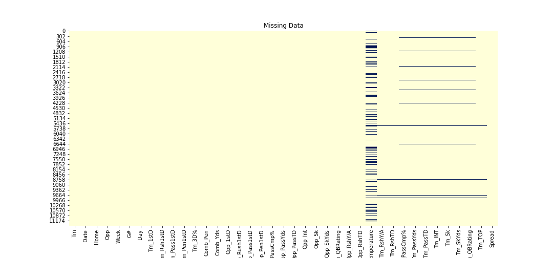
3. The third step we took was to impute missing values in columns that contained missing data. We did this by randomly sampling from the column with missing values and randomly placing them in the column. Most of our columns had a relatively low amount of missing values, therefore by doing this we are not compromising the integrity of our data. Below is a heatmap representing which columns were imputed in our dataset.
4. The fourth and final step in data cleaning was to remove outliers. We did this by using the common rule of thumb which is 1.5 times the Interquartile Range (Quartile3 - Quartile1). This is reasonable because it is very uncommon for an NFL game to end with a Spread larger than 35 points, therefore keeping this data is doing nothing more than adding bias to our model. Below we can see that by using this rule, we are removing a minimal amount of data.

4.Exploratory data analysis

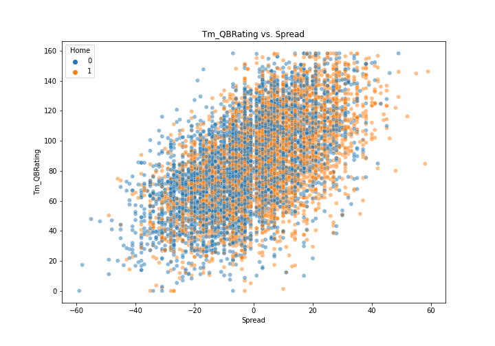
In our exploratory data analysis, we created histograms of each of our variables to understand any skews in our explanatory variables. Additionally, we made scatterplots with each of our variables and our response variable, Spread, to see if we can observe any strong relationships prior to building our model. Most of our variables were non-linearly related with Spread and required a model that can find interactions between variables in our data in order to accurately predict Spread. However, the performance of the QB on both teams showed the most correlation with Spread when analyzing the explanatory variables individually with Spread. In the plots below, we can see that the higher the QB rating of the team in the “Tm” column, the Spread tends to favor them, and vice versa. The worse the “Tm” QB does, the spread favors the “Opp”. Using this information we are able to understand that this will be an important feature in our model.

5.Building Neural Network ML Model

5.1 Baseline model

To generally view the linear relationship between different stats of match and the score spread, we build a simple linear regression model. The summary of the baseline model is shown as below.

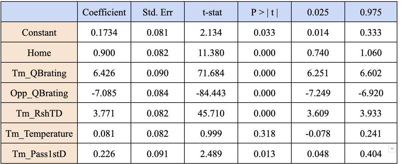
The ordinary least square linear regression model estimates showed us that the team quarterback rating has a strong positive linear relationship with the score difference and the home feature seems not that important. This model is by no means a strong predictor of spread, however it helped us gain a stronger understanding about the relationships in our data going forward.

We also notice that the OLS linear regression model did not capture a strong linear relationship with Temperature and Pass1stD with Spread. We think that there are more of our features that we can not perfectly capture their relation to the score differences simply by linear regression estimates. Therefore, we decided to develop an N-N model to have more accurate predictions since it can capture the non-linear relationships and interactions in the data.

5.2 Multi-layer Perceptron Neural Network Model

At first, we had 34 features as input for a MLP regressor model using relu as activation function , but unfortunately the performance was bad. Even though the training error and test error was low, the real prediction for 2022 Super Bowl Prediction, as well as our validation set predictions, were not even close.

We collected the features of the 2022 Super Bowl match and the prediction value varied a lot with even negative spreads which is completely opposite to the real result:

Los Angeles Rams defeated the Cincinnati Bengals in Super Bowl 2022 with the score 23-20. Our model at this phase was not robust at all, we kept getting results like +80. +120, -34, -6 which vary from the actual +3 a lot.

5.3 Feature selection

Before tuning hyperparameters, we did feature selection first to improve the performance.

We subtracted “Tm” stats from “Opp” stats and created a new set of features. This brought us down to 16 features. With this reduction in features the prediction was a little more reasonable as the real predictions ranged from -5 to +60.

Additionally, the testing error (MAE) also reduced from 6 to 4, but it was still not robust enough, so we needed to tune different hyperparameters.

5.4 Hyperparameter Tuning

We definitely experienced some hartim while tuning the hyperparameter because there are so many parameter we can change like activation function, hidden layer size, neurons size.etc

Below is a table that briefly summarizes some of the hyperparameter combinations that we tried.

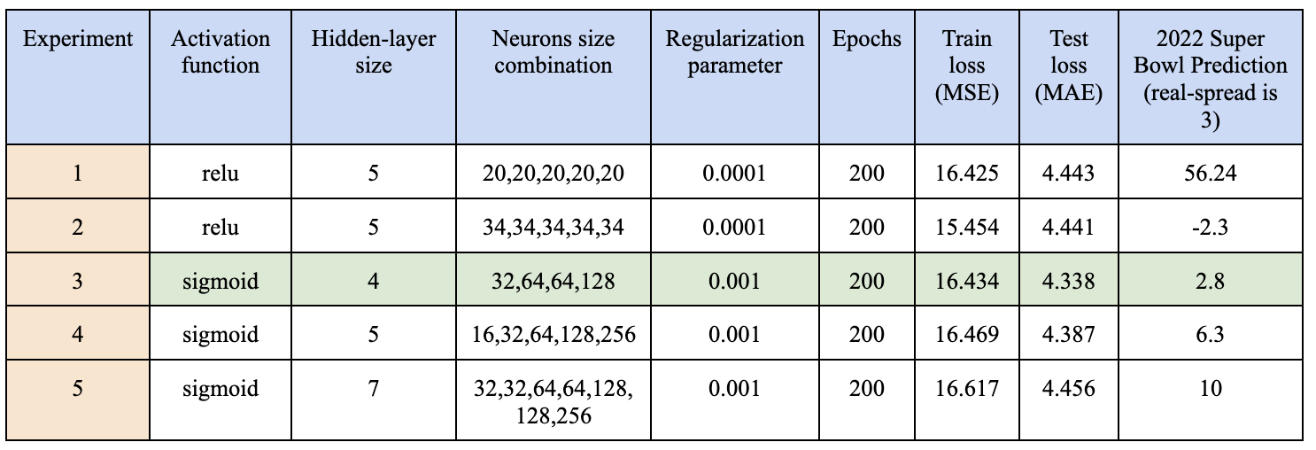
As you may have noticed, the sigmoid activation function is better for our NFL predictions and since we have around 10,000 data points, the hidden-layer size shouldn’t be large, to avoid overfitting. Experiment 5 actually resulted in higher errors compared to others with smaller hider layer size. We also surprisingly found that 2ⁿ neurons in each hidden layer performs much better than other random numbers.

After trying out tons of hyperparameter, we finalized our MLP-Regressor model : with 4 hidden layers and a neuron size combination of (32, 64, 64, 128)

The maximum epochs (how many times each data point will be use) of the model setting is 200 since the loss curves at blow showed us the training loss stopped decreasing around 80 epochs because the validation loss started to increase at that iteration.

The validation data was set to 20% of the training data.

5.5 Test Robustness

To test the robustness of our MLP model, we tried different initial values of weight and bias by changing the parameter of “random_state” in scikit-learn MLP regressor package.

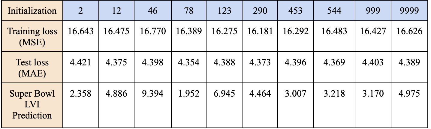
After trying out different initial values of weight and bias we can conclude that our model is robust since the training error, test error, and prediction for the super bowl this year did not have large variance. In the real world, our averaged prediction among these 10 different initializations is 4.437 which is very close to the real value 3. .

5.6 Permutation Importance Analysis

With this final model, we started to inspect the importance of all features by performing a permutation importance analysis on this Neural-Net Model.

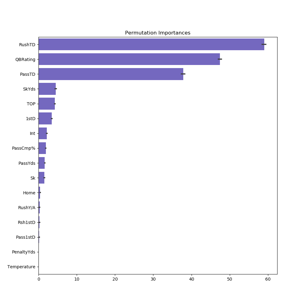
This analysis measures the decrease in model performance when shuffling an individual column. This randomly shuffled procedure breaks the relationship between the feature and the predicted value, therefore the drop in performance is indicative of how much the model depends on the feature.

According to our permutation graph, RushTD , QBRating, and PassTD are the three most important features. It also agrees with what OLS linear regression estimates’ results that Temperature, Pass1stD, etc has little explanation of Spread.

We should always keep in mind that permutation importances does not reflect the intrinsic predictive value of a feature by itself but how important this feature is for this particular MLP regressor model.

Although we have shown that this model performs extremely well, we still want to do further research like correcting the statistical inference on the relationship between the selected features and the game spread.

6.Applying Post-Prediction Inference

The permutation graph shows the importance of each feature to the prediction model, but in order to accurately gauge the effectiveness of postpi on inference correction for our data we must apply postpi to each of our covariates, later on in our results we will feature our findings for two high importance features (RushTD and QBRating) and two moderate/low importance features (TOP and 1stD). First, some definitions of what exactly postpi is. Postpi is a method for improving statistical inference by correcting model bias and improving variance estimations. Model bias refers to the difference between average prediction and the correct observation the model is attempting to predict, high bias is due to an under-fitted prediction model and leads to high training/testing error. Variance estimation relates to a model’s ability to predict on testing and unseen data, high variance is due to over-fitting on training data and leads to high test error.

Statistical inference (and the strength of the inference) refers to the analyst’s capactiy to derive a trend or relationship between a covariate of interest and the outcome in a sample population, and then apply it to the entire population.

A hypothetical example to help understand this in the context of sports analytics is a “Home Field Advantage Inference” example. A sports analyst takes a random sample of NFL games and finds statistically significant results that a team playing on its home turf has around a 10-15% higher chance of winning. Because of the analyst’s strong findings, they can provide reliable statistical inference across all NFL games (future or otherwise) that a team playing on their home turf has around a 10-15% higher chance of winning.

Now that we have some key definitions explained, we can move onto the actual implementation of postpi. With our well tuned prediction model ready for use, we apply it on the test set to generate a list of predicted and observed outcomes. A key aspect of post inference correction is producing a low dimensional (in our case linear regression) model to capture the relationship between the test set’s observed and predicted outcomes. We will later on use the relationship model to simulate “observed outcomes” by plugging in predicted outcomes and returning corrected predictions. Inference correction by altering the prediction model would be possible for a simple model, however it would be nearly impossible to conduct meaningful improvement by altering a highly complex model such as MLP Neural Networks.

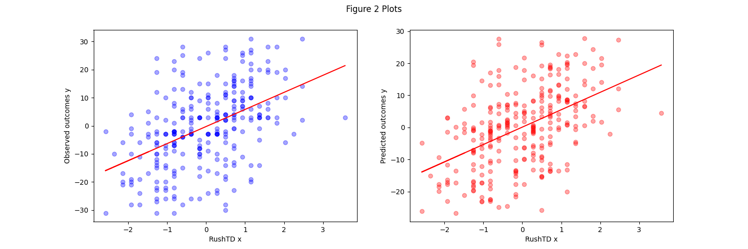
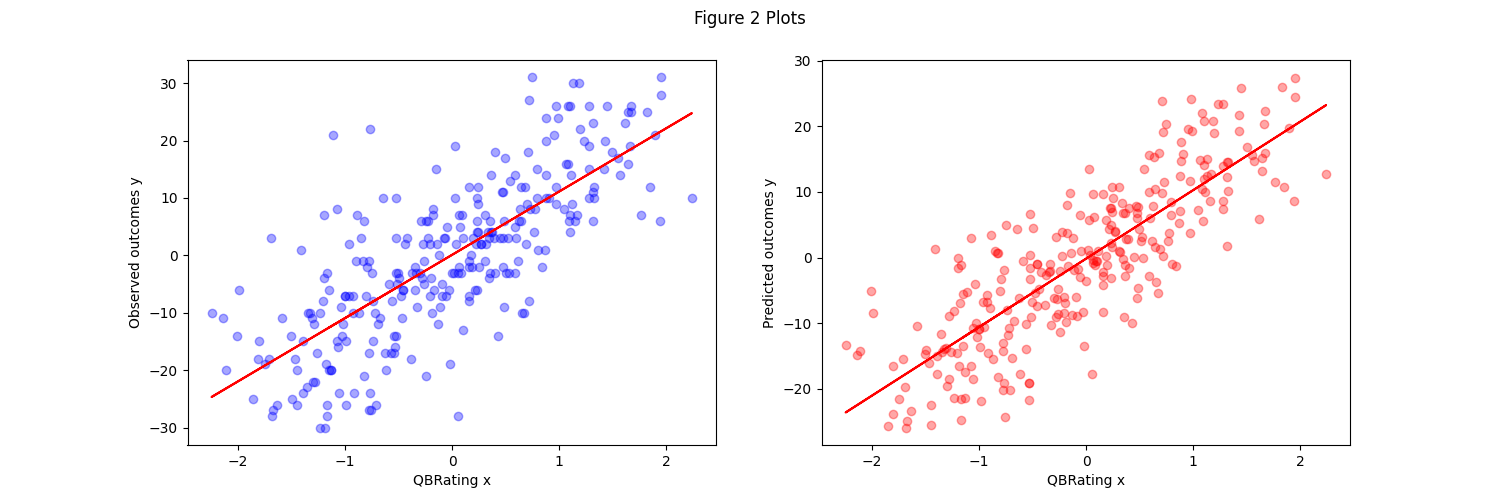
Here we highlight our findings thusfar on our aforementioned four covariates of interest. The first set of graphs compare the covariate of interest to the observed and to the predicted outcomes. You’ll see that for all 4, the predicted outcomes share a very similar relationship to the observed, but do tend to show less variance and more bunching near the central lines.

RushTD

QBRating

TOP

1stD

In the next set of graphs we compare the relationship models generated on each covariate of interest from the NN and baseline (linear regression) models. You can see that despite the complexity difference between neural network and linear regression, they all successfully generate a linear relationship between the observed and predicted outcomes. Furthermore, it’s clear to see that the MLP NN does a far better job across the board at capturing the relationship as the linearity is much stronger.

RushTD

QBRating

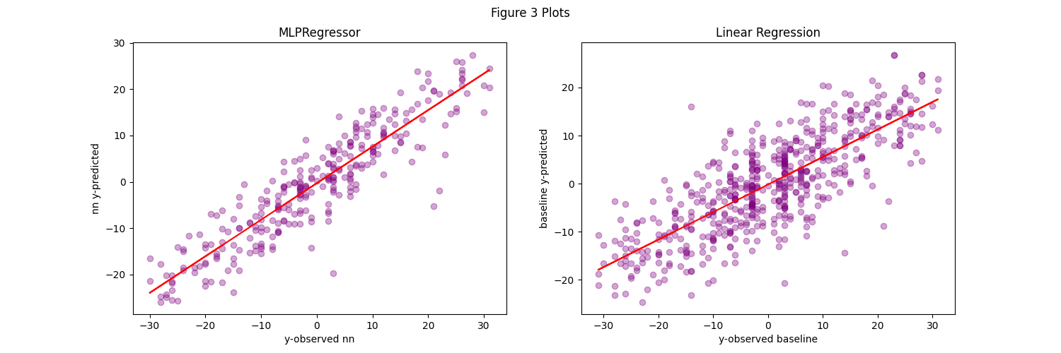
TOP

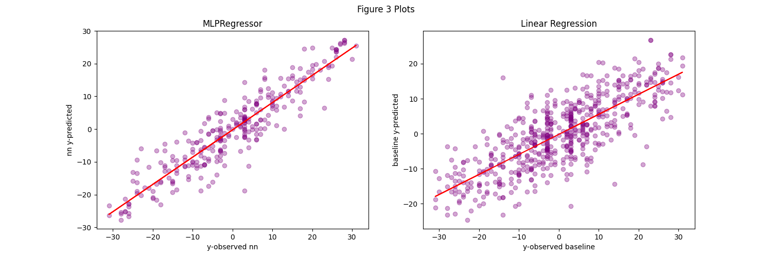
1stD

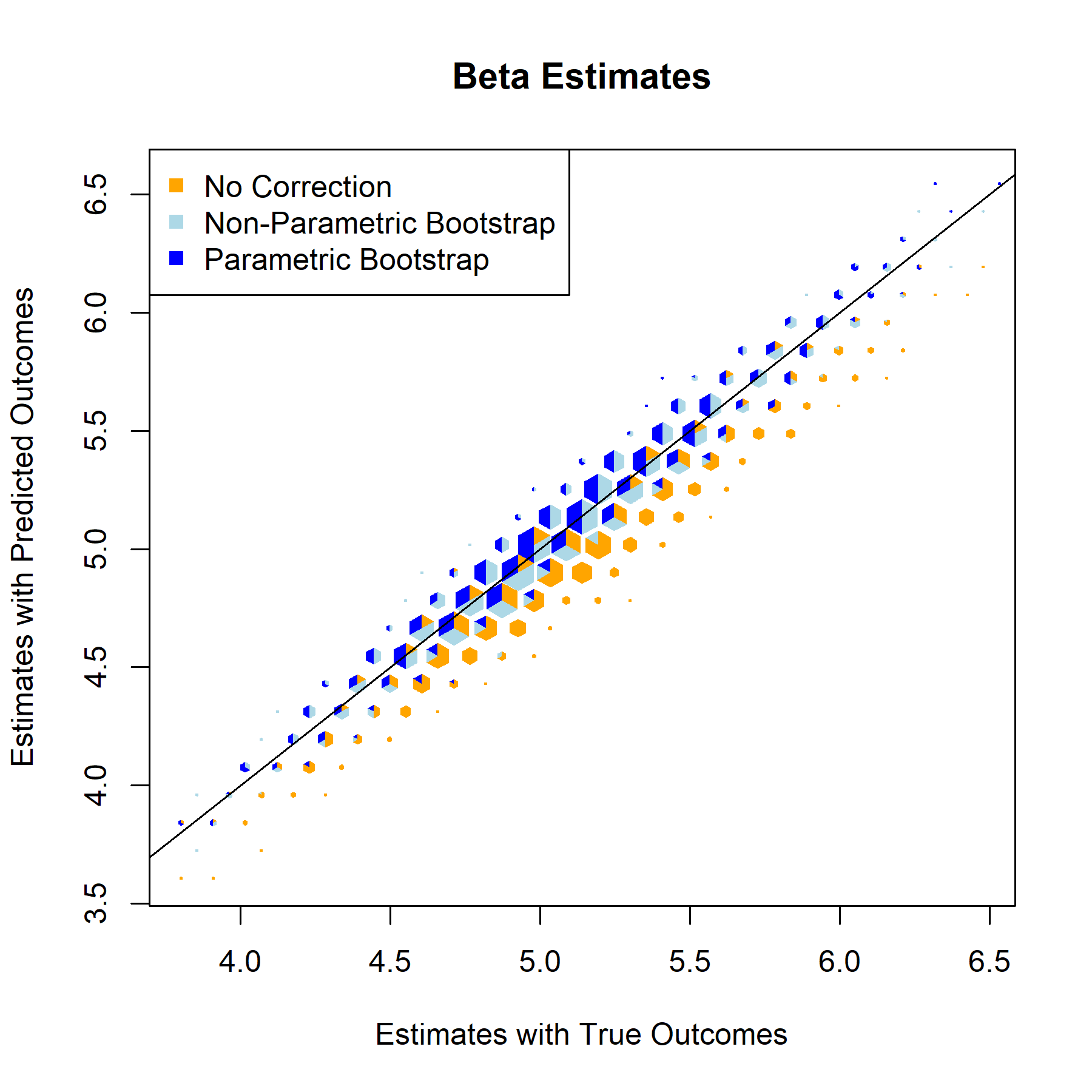
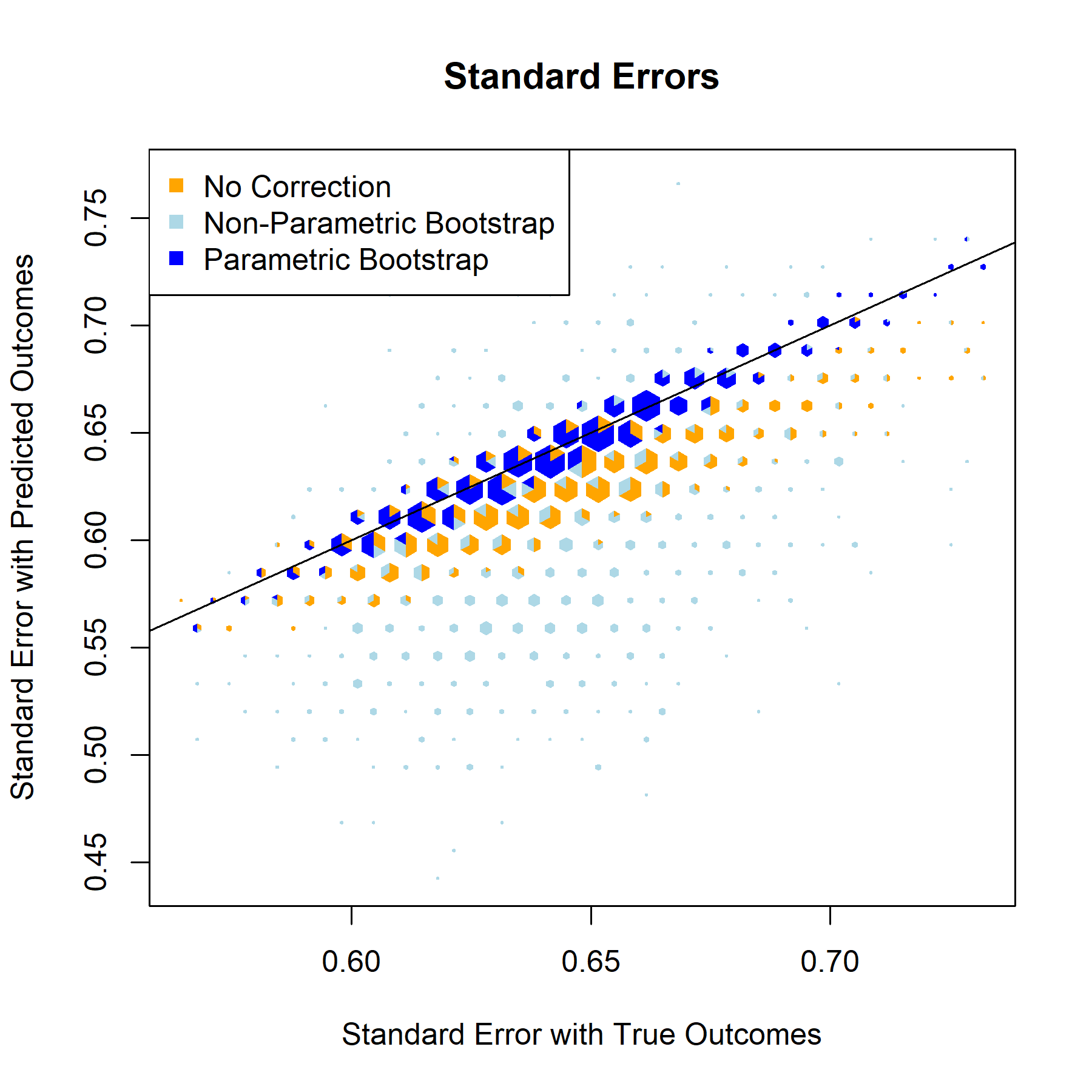
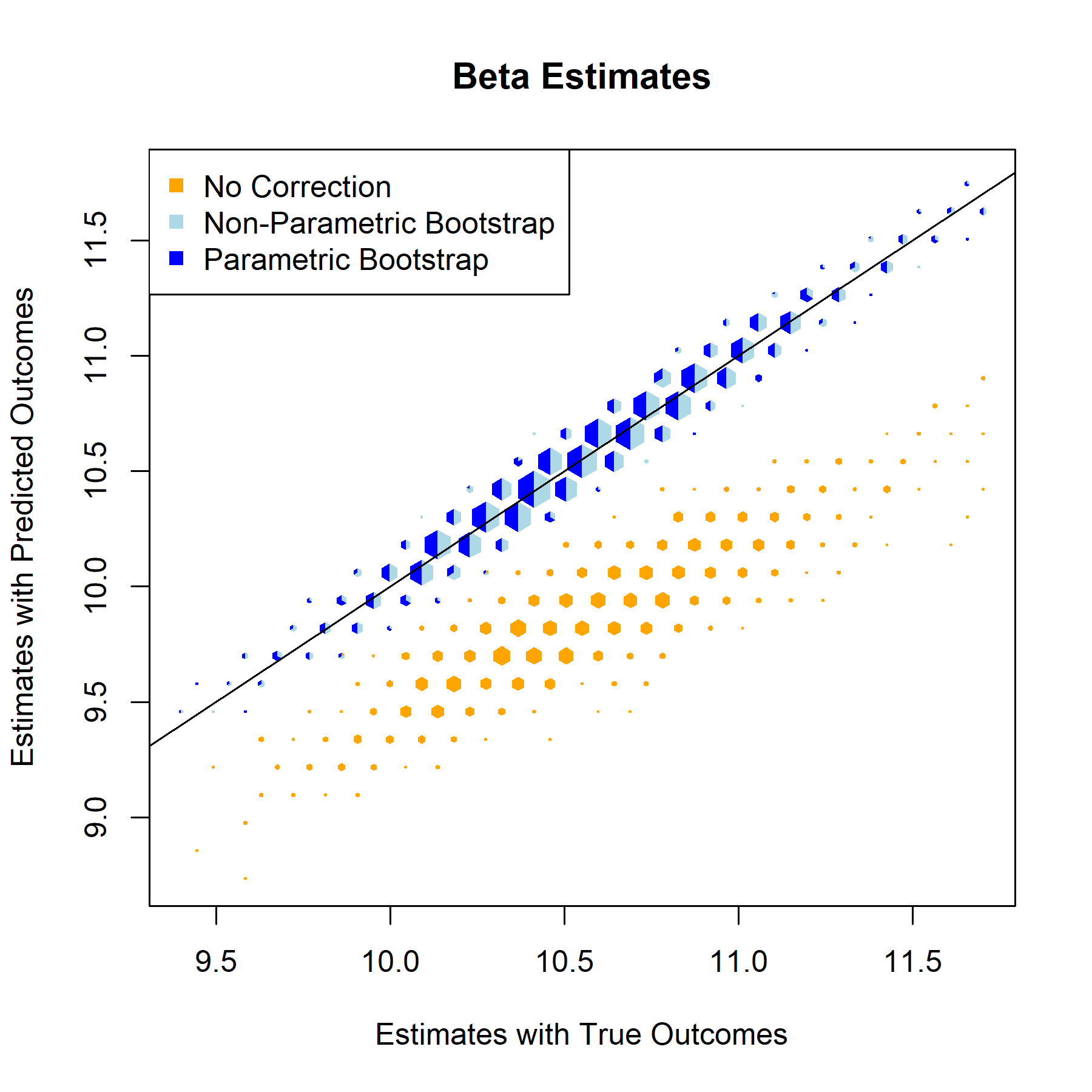
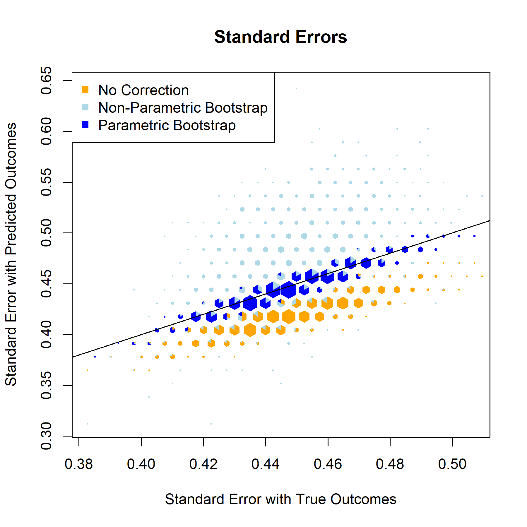
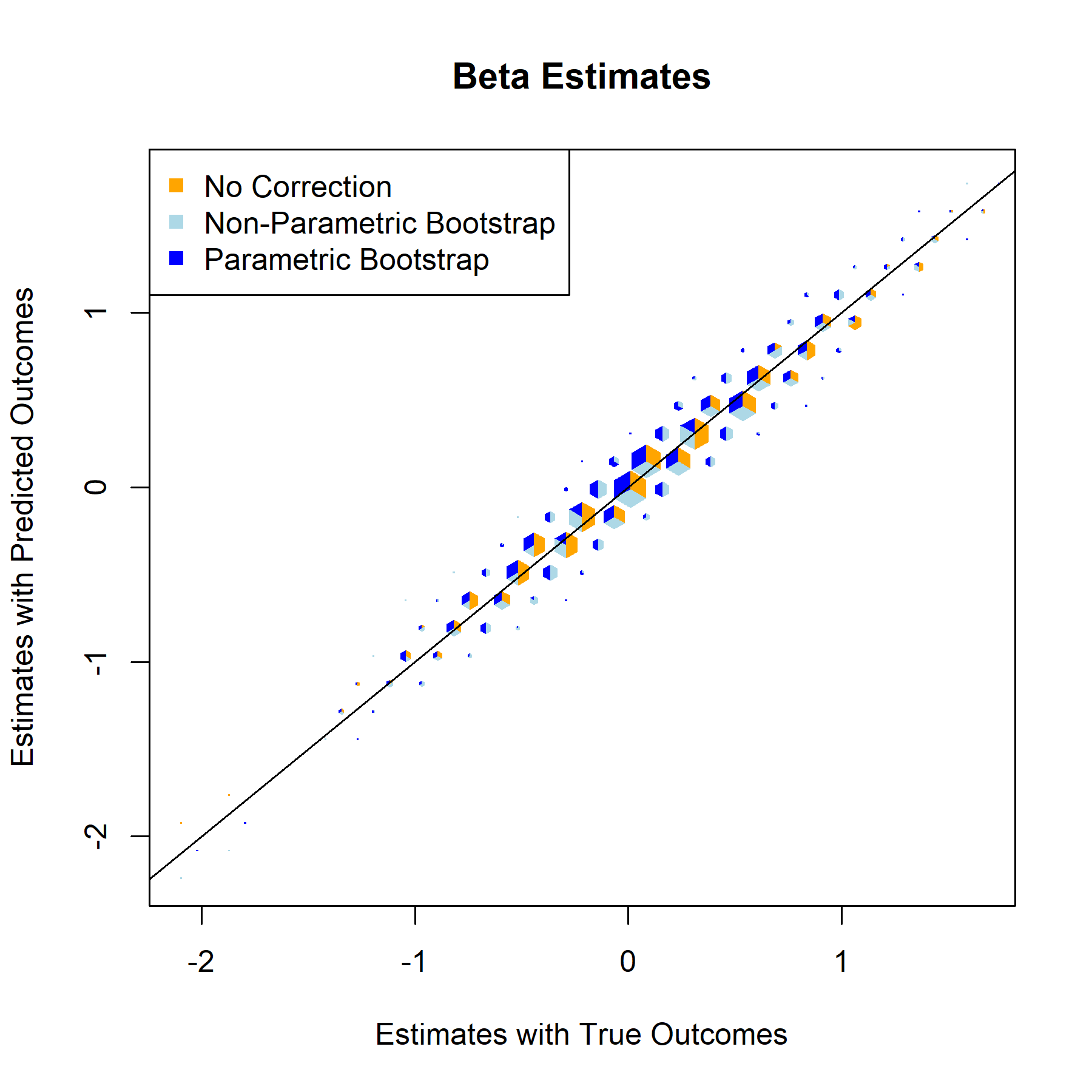
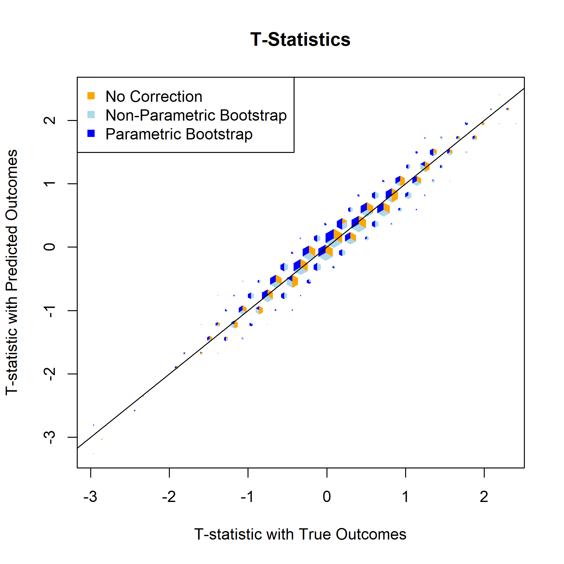
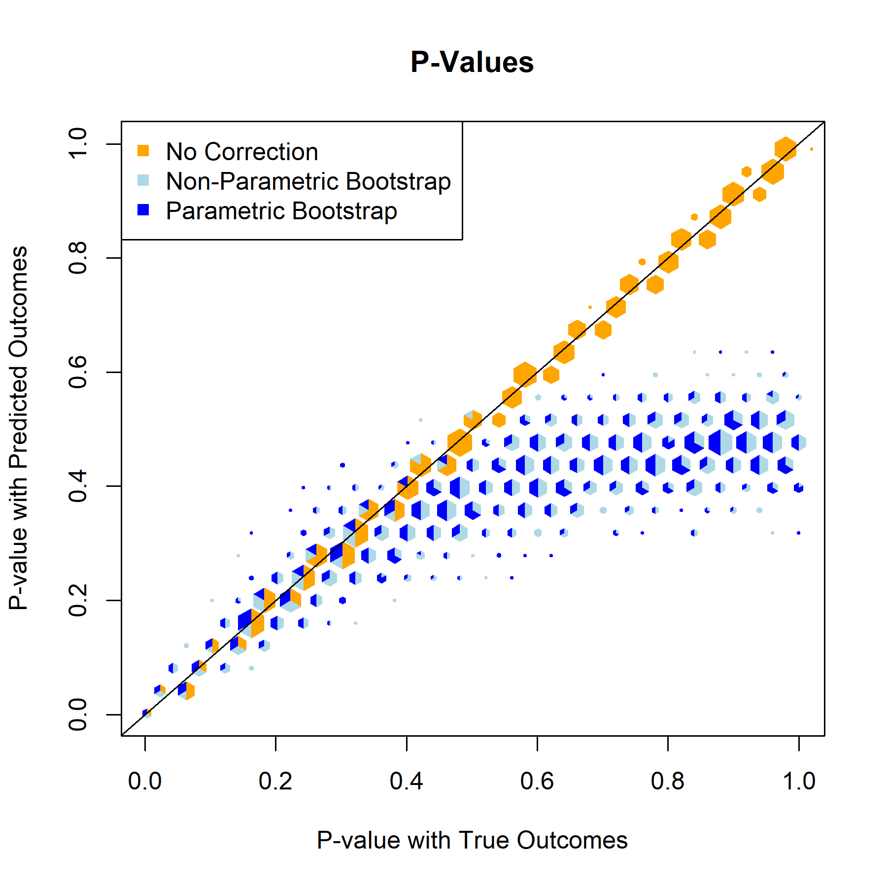
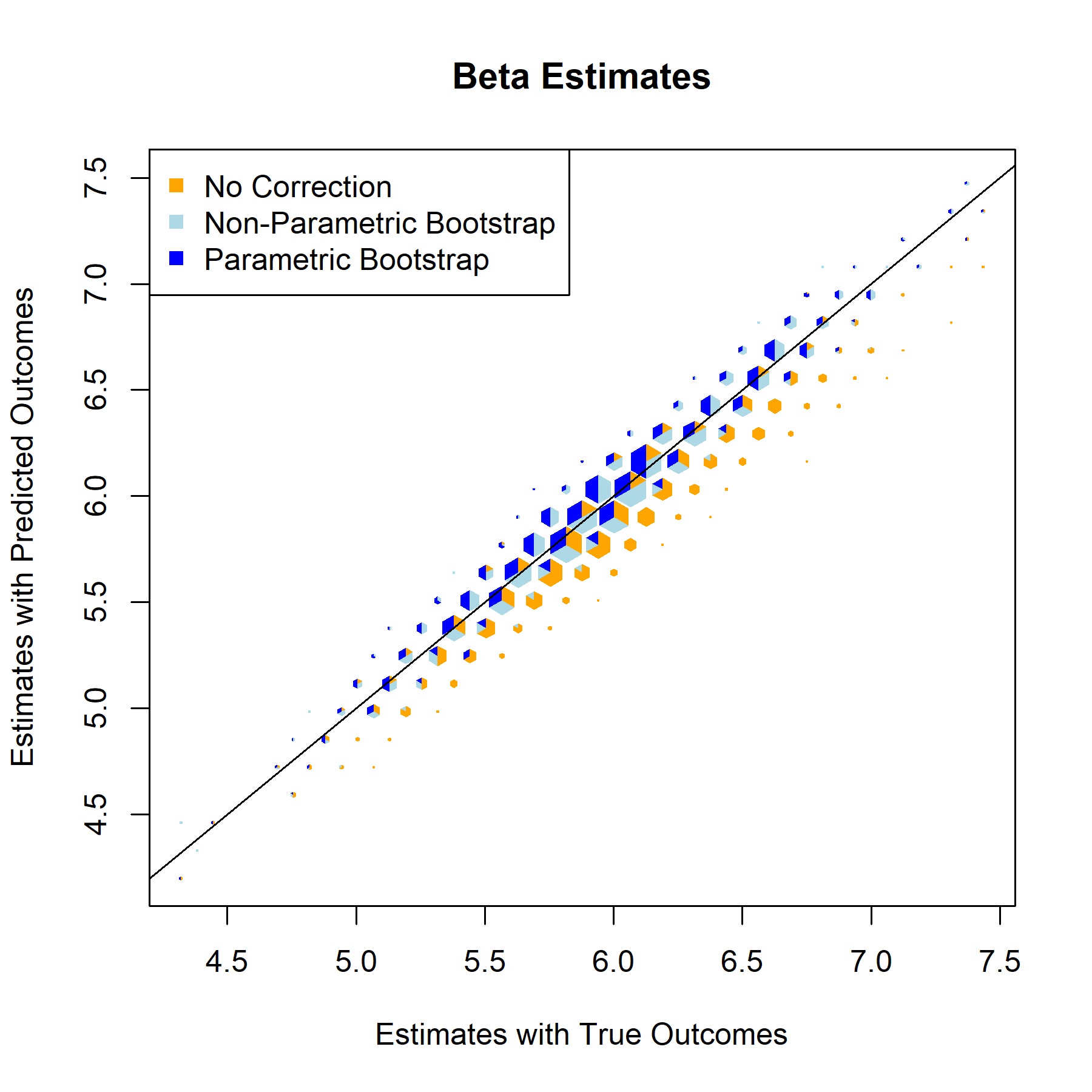
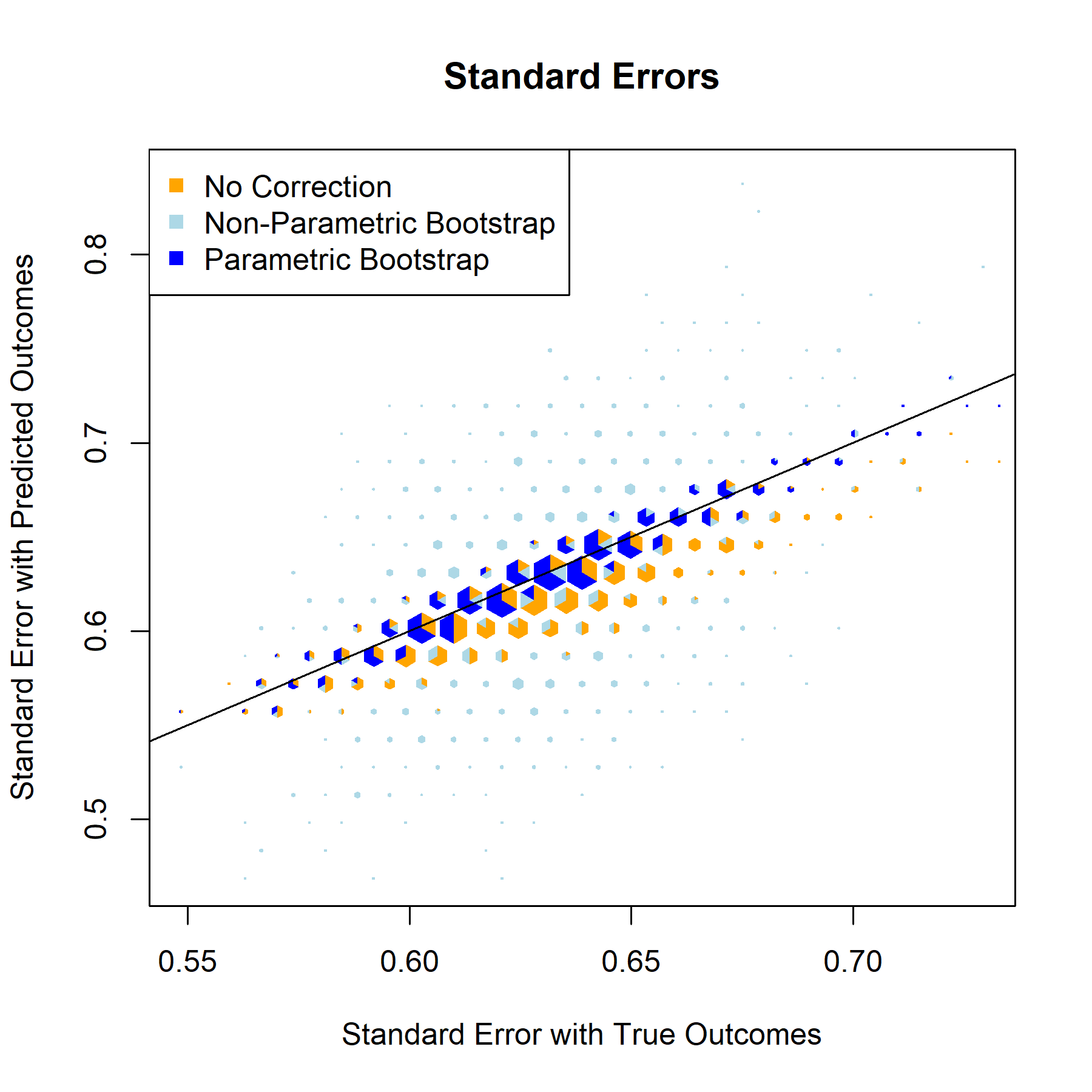
Having established that the relationship models are strong and function as expected, the next step is implementing bootstrap based correction on the validation set. The bootstrap repeatedly samples from validation data to better represent the entire population, generates an inference model for each iteration, and returns aggregated metrics for the inference models’ corrected beta estimates, standard errors, test statistics, and p-values.

RushTD

Beta Estimate

Standard Error

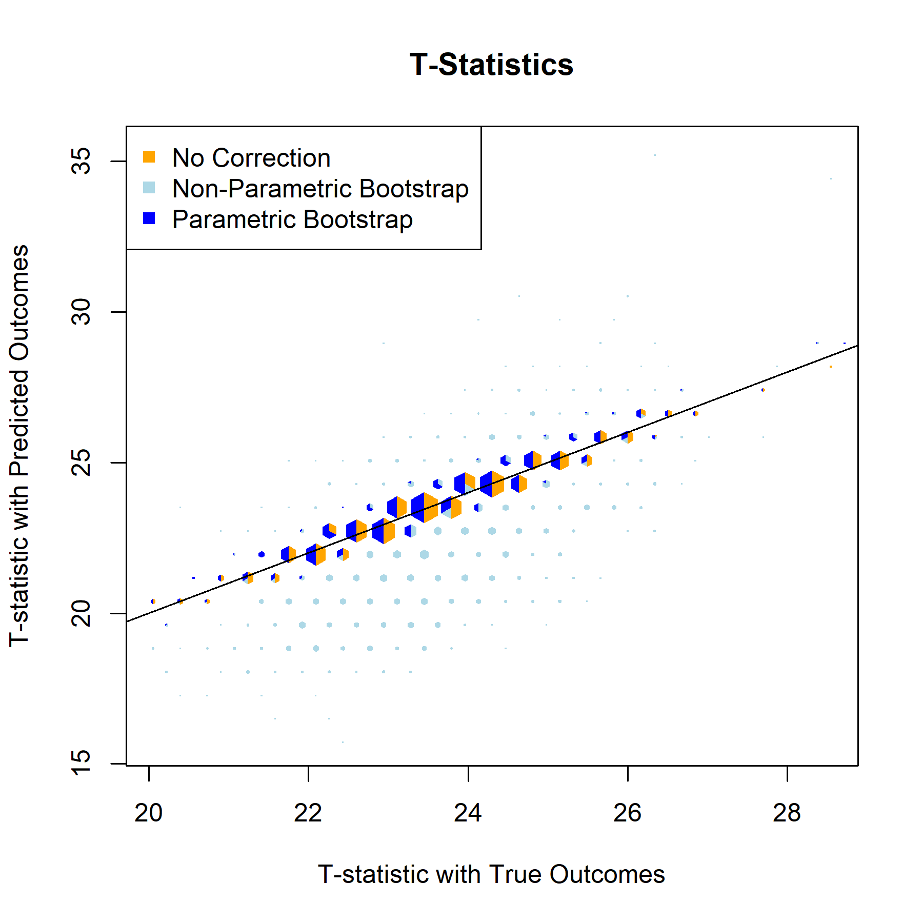
T-Statistic

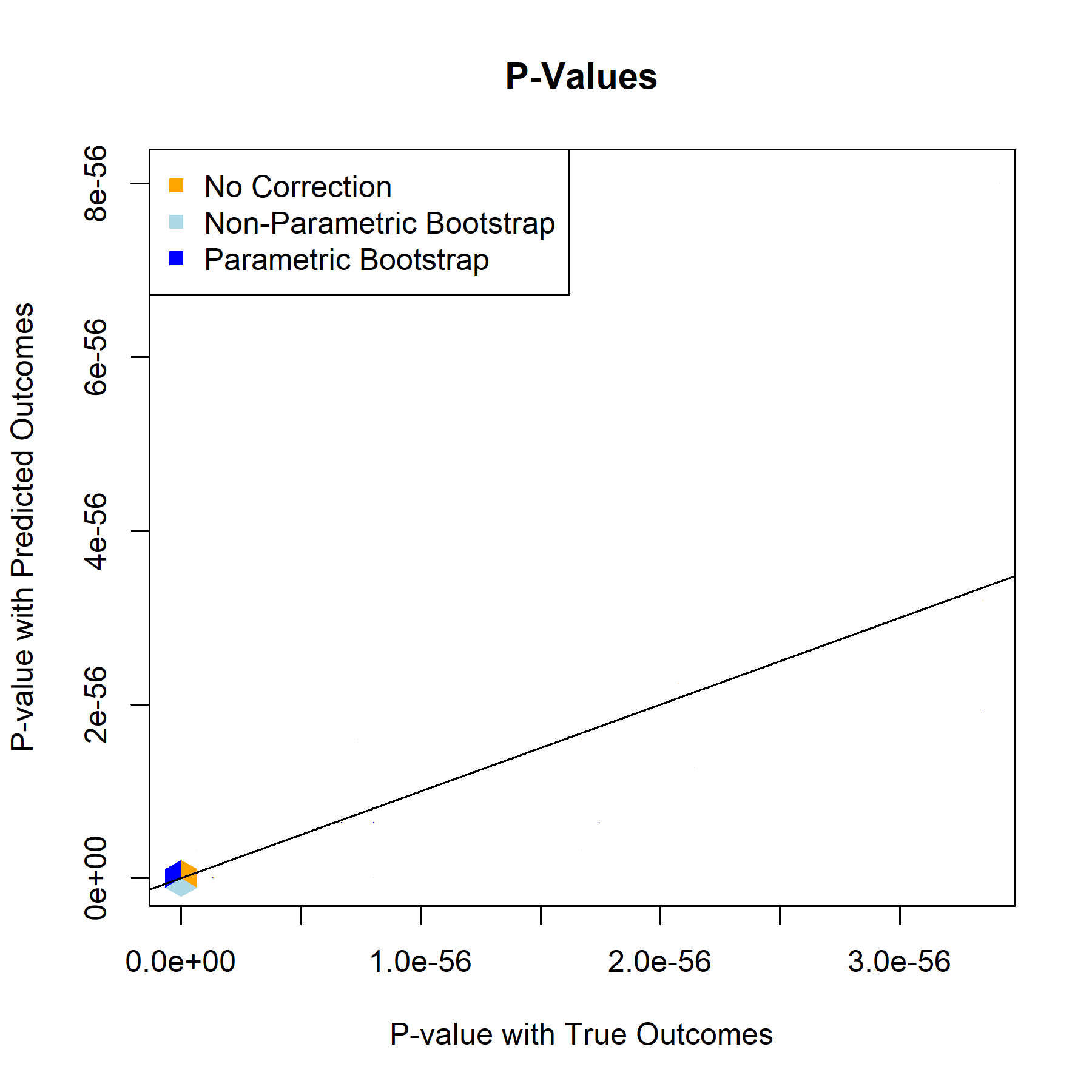
P-Value

QBRating

Beta Estimate

Standard Error

T-Statistic

P-Value

TOP

Beta Estimate

Standard Error

T-Statistic

P-Value

1stD

Beta Estimate

Standard Error

T-Statistic

P-Value

Results

For every one of the featured covariates (and indeed for all of the covariates in our data set), the T-Statistics and P-Values graphs provide a clear answer to the to the question “to what degree, if any, will postpi provide statistical inference correction for our NFL sports analysis?” The answer to that being “not much”, apparently.

7.Conclusion

In conclusion, our project followed all the steps of a data science project. We began with collecting our NFL game data and compiled a final dataset by using all the different smaller datasets we collected. Then, we conducted exploratory data analysis to understand the relationships between variables in our data, and dealt with common pre-processing steps such as missing values and outliers. Once we had a strong understanding of our cleaned dataset, we built a simple linear regression model as a baseline to improve on to gain some understanding on how our covariates impact our response variable, Spread. Once we saw that our baseline model is not capturing all the relationships in our data, we developed a neural network model that performed much better than our baseline model. With this model we were able to achieve a near perfect prediction on Superbowl LVI, and an average error of 4 points, nearly half of our initial baseline model. We then set out to understand the importance of each of our features so that we can apply our research of post-prediction inference to better correct our inference on these variables. After using the method of postpi, we find that our neural network model results in a very accurate representation of our covariates, and therefore we can speculate that due to this statistical inference correction is not necessary in this case. Our post-prediction inference methods helped confirm that our model is quite accurate in inferring the relationship for each of our features that is used to determine the outcome of an NFL game.

https://jonlangley2022.github.io